One of the frequent topics on the Systematic Investor podcast concerns volatility targeting or volatility scaling. There have been vivid discussions on various episodes, sparked by current research, such as the excellent paper by Campbell Harvey et al. ‘The Impact of Volatility Targeting‘ and the often cited paper by Moreira & Muir on ‘Volatility managed Portfolios’. The papers make valid points regarding the mechanism and impact of targeting a fixed volatility for your portfolio. Amongst the findings there is the following statement:
Volatility scaling reduces the likelihood of extreme returns, across all asset classes. Particularly relevant for investors, “left-tail” events tend to be less severe, as they typically occur at times of elevated volatility.
C. Harvey in ‘The Impact of Volatility Targeting‘
This does not come as a surprise, as statistically speaking volatility is not only time-varying but also:
- asymmetric: volatility is higher in times of stress (negative returns) than in times of calamity (positive returns)
- clustered: the volatility changes over time and its degree shows a tendency to persist, i.e., there are periods of low volatility and periods where volatility is high.
Benoit Mandelbrot described this first in 1963 in ‘Variation of Certain Speculative Prices‘.
These and other aspects of volatility gave rise to a variety of statistical models with fancy names such as ARCH, GARCH, ARFIMA, their multivariate counterparts MGARCH, DCC, VARFIMA (don’t forget about correlations!) and even nonlinear dependency measures. For anyone who is interested, I dived into that topic a while back in my dissertation.
But don’t worry, today’s subject will be much simpler, namely:
Why do Trend Followers dislike volatility targeting?
Niels, Jerry and Moritz have all raised their concerns regarding the usefulness of volatility targeting for Trend Following portfolios on the Systematic Investor podcast. Based on their comments, there are three major concerns that come to mind:
- It’s not based on individual position risk but portfolio risk. As a result, the riskyness of one trade in your portfolio has a big impact on other potentially unrelated trades. It is not only confusing in terms of risk management, but also destroys the intention of Trend Following: letting winners run and cutting losers short. As a result of volatility targeting, an increase in portfolio volatility can lead to a ‘dampening effect’, meaning you have to scale down winning positions.
- Volatility is a symmetric risk measure. Hence, your volatility might increase even though the ‘risk’ of your position does not increase. This is less problematic for volatility targeting on long/neutral portfolios as for them, times of high volatility are indeed correlated with negative returns. However, a long/short Trend Following portfolio might make significant positive returns from short positions in volatile markets. Again, these would be scaled down. Note that is essentially true for any symmetric risk measure.
- Volatility targeting is not free of costs: You have to calibrate the speed of adjusting your portfolio or apply a more sophisticated trade count optimization to bring costs down to a tolerable level. Instead of adjusting the position that carries the most risk, you might have to touch all your positions. This can be useful in case your positions are all positively correlated (again, maybe for a long only equity portfolio), but lead to unnecessary trading in long/short multi-asset portfolios.
To illustrate some of the effects, I decided to look at a Trend Following (TF) strategy to which I apply a target volatility mechanism. The strategy is a long/short Donchian channel strategy with individually sized positions on 40 futures markets (equities, bonds, currencies and commodities). The strategy takes into account trading costs and slippage.
The total return of the strategy looks quite reasonable as illustrated below (Sharpe Ratio ~ 0.83). As expected for a Trend Following strategy, annualized volatility might be higher than some people might like it (35%).
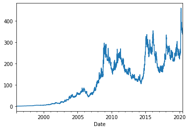
Total return of the unscaled Donchian channel strategy.
If we compare the 3-month returns of our TF strategy against the 3-month returns of the S&P 500, we can observe the convexity of the strategy relative to the S&P (follow this link for a more detailed discussion of the convexity of Trend Following). In ordinary words this means that persistent and cumulatively large moves in the underlying produce big returns for the strategy. In this case our strategy does not simply trade one underlying, so our convexity is a little bit ‘blurred’ but still visible.
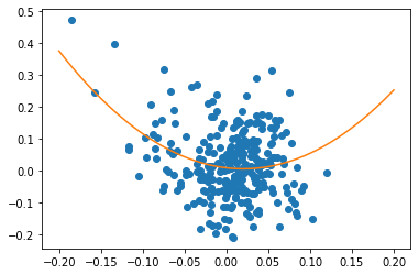
x-axis: 3-month S&P 500 returns, y-axis: 3-month TF strategy returns.
Orange line is a second degree polynomial to illustrate convexity.
Also, the return distribution is slightly positively skewed (+0.10), meaning that our losing returns are smaller in magnitude than the winning returns and we have a high proportion of relatively poor returns (see this blog post by Rob Carver for an excellent article on TF skew).
So, what happens to these characteristics once we apply volatility targeting? For this exercise I use a 90 day window to estimate rolling standard deviations and scale the returns to an annualized target volatility of 10%, a number which is much more convenient for most investors. I implement a leverage cap of 150%. The position adjustment is lagged by one day, based on the assumption that the volatility targeting trades are implement on the next day’s close.
As a result of the vol targeting, the strategy’s Sharpe Ratio does increase slightly to 0.87, while the CAGR decreases from a whopping 27% to a more behaved 9%. The positive skew of the strategy decreases from 0.10 to 0.023. Correlation to the S&P ‘only’ increases from -0.18 to -0.11, but these numbers must be evaluated with some caution. Since correlation is a linear measure of dependence and the above relationship between the strategy’s returns and the S&P 500 is clearly nonlinear, a better way to look at the impact of vol targeting is again the plot of strategy returns vs. S&P returns below.
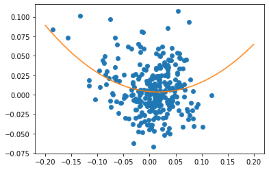
x-axis: 3-month S&P 500 returns, y-axis: 3-month volatility scaled TF strategy returns.
Orange line is a second degree polynomial to illustrate convexity.
While we can still observe convexity many of the data points to the left move down the y-axis. Where the strategy returned around +25% to +48% while the S&P 500 lost -15% to -20% on a three month horizon before, it is now more in the region of 5% to 10%. This clearly shows the impact of vol targeting mentioned above in point 1. and 2. Despite winning positions during the times of market turmoil, exposure to these positions is decreased due to an overall increase of portfolio volatility.
There are definitely some good reasons for volatility targeting, e.g. bringing portfolio volatility in line with expectations and making risk more endurable for investors. However, for a Trend Following portfolio part of the strategy’s favorable characteristics are destroyed in the process of aiming for a fixed volatility target. If you want to keep convexity and positive skew alive, volatility is part of the game.