Last week’s market action seemed pretty unrelated to my daily doings at first, but had a lasting impact towards my thinking in the end. Equities, allegedly driven by “dumb money” showed a lot of optimism following the easing of lockdowns around the world as many of my friends proved me wrong in my hesitation to buy the dip. Even Goldman Sachs revised their gloomy outlook on stocks, despite Corona continuing to have a massive impact on global economies, as this recent research paper from the United Nations puts it:
While advanced economies are expected to be hit hardest by the COVID-19 crisis, two emerging regions will also suffer above-average declines: developing Europe and Latin America and the Caribbean.
As an addition, there have been protests in 75 cities across the United States as well as other cities all around the world after the killing of George Floyd in Minneapolis. The market didn’t care. Why? This article points towards the amorale nature of the stock market as one of the reasons. Another quote from the article that I find interesting is this one:
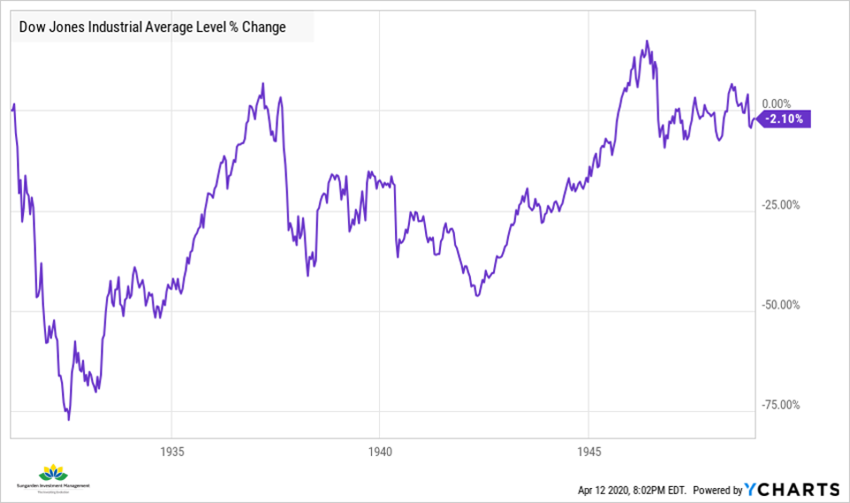
David Rosenberg, who runs a market research firm in Toronto, argues emphatically that whatever the short-term movements of the market, major declines and an extended economic struggle will be coming. He compared the current rally to the rebound that began in November 1929 and lasted until April 1930. The market gained almost 50 percent in that period, he said, but no one remembers it. What we remember is the Great Depression.
So, what came after the rebound in 1930? You can find a very nice summary in this article. The quintessential point is:
The market regains its old 1931 peak…a generation later!
I don’t want to make any predictions at this point, as these are most likely wrong…maybe even as wrong this week’s unemployment estimate. Just a tiny 10 million jobs miss by analysts on May Non-Farm Payrolls (exp. -7.5mm vs. act. +2.5mm). However, as a statistican, forecast error has always been part of the game of trying to guess estimate future developments and we should probably not overestimate single predictions.
Ok, so far so good. Uhm, well … Despite being mostly systematic, I actually do care about what’s going on, but it should not influence my investment decisions. So all is good…or not. I actually wanted to know what made some of the people I know so confident in buying the dip. These were mostly guys who never touched financial instruments before and called me when the crisis unfolded to inquire about the cheapest way to get into the action. Of course, I urged them to be cautious, think about the risk potential and not making any hasty decisions because stocks seemed so cheap. I knew that none of them had any money problems, so I tried to help them to size their positions reasonably and take a few bets. What I did however miss at that point was the question about their motivation. Where did the buy the dip mentality come from?
One of the insights I got was that actually none of them believed in a quick recovery and most of them showed signs of FOMO. So, I tried to get a little bit deeper and asked them about their return expectations and the horizon they are willing to hold on to these positions. And that’s were things actually got more interesting: Most of them used retirement simulation tools provided by automated investment advisors (robo-advisors) to get an estimate on how bad things can turn out and what to expect for the future. As a disclaimer, I worked for a robo-advisor before. We used to build tools to make sure people will have reasonable estimates of their retirement income and necessary savings. Apparently these were not the ones my friends were looking at, since we included some reasonable estimates. My friends however showed me graphs with 8-10% annual performance estimates for long only equity strategies. There was only one reasonable reaction: Heavy doubt. Don’t get me wrong. I’m with anyone who can afford it and bought the dip to hodl his way to financial success, but I’m highly sceptical of inflated estimates on future wealth. It’s not only about the size of your return estimate, but rather the estimator itself.
Let me bring back some statistical knowledge about the estimation of future wealth, which might in the end be +- 10mn off anyway and which I mostly gained from a working paper co-authored by my brother: “Forecasting Final Wealth By Mean, Median, or Mode?”.
Forecasting final wealth is ugly. Not only do your return and volatility assumptions matter a lot, forecast also have to tackle the extreme skewness of the distribution of final wealth. There is a very nice paper on the misuse of expected returns by Hughson, Stutzer and Yung which shows that the density function of final wealth (after 20 to 30 years) is extremely skewed to the right:

This is also visible in final wealth simulators that use interval forecasts for final wealth. However many places still use the expected value of final wealth as a point forecast because it minimizes the expected squared forecast error. This could indeed be a reasonable choice if the probability distribution is symmetric and not heavy tailed. Nevertheless, forecasting the final wealth by the expected value is far too optimistic (see the mentioned paper above) even assuming only i.i.d. (Independent and Identically Distributed) returns. If we assume that people doing these long-term forecasts are (hopefully) using a long history of data, it’s very likely that their estimates are based on monthly or yearly values. So, the i.i.d. assumption make sense considering the input.
The paper also looks at heavy tailed distributions. This even leads to cases where the expected value of final wealth is infinity despite a symmetric distribution (e.g. Student-t) . As much as you would like to have infinite wealth within your retirement horizon, you should be highly sceptical if an advisor suggests this.
Now let’s talk numbers and look at a simple solution from the papers: Just use the median instead of the mean to estimate final wealth.
Based on two different historical periods (1959 – 2016 and 1987 – 2016) and retirement periods of T = 10, 20 and 30 years starting in 2016, the paper arrives at the following values for the DAX 30 Index:
| Period | 1987 – 2016 | 1959 – 2016 | ||
|---|---|---|---|---|
| Planning Horizon | Median | Mean | Median | Mean |
| T = 10 | 2.09 | 2.82 | 1.74 | 2.21 |
| T = 20 | 3.57 | 6.47 | 2.77 | 4.48 |
| T = 30 | 4.96 | 12.11 | 4.07 | 8.36 |
Assuming a wealth of 1 at the start date 2016 and a historical volatility of 0.244 for the period starting in 1987 and 0.219 for the period starting in 1959. Unbiased estimators for median and mean are used.
Using the improper estimator leads us to overestimate the final wealth by a factor of more than 2 over the 30 year horizon and 1.6 to 1.8 over the 20 year horizon depending on the historical data used for estimation. Note that if you use other historical periods (very short and very unfavorable), it’s not guaranteed that you end up with any wealth at all.
Oh boy, my retirement crisis golden years looks awesome! #happytrading and don’t forget to buy Bitcoin. #notinvestmentadvice